Basic Raytracer in C++

Computer graphics has always felt like a magic to me, which I was distantly approaching from different sides, yet haven’t been getting close enough to. Once I’ve realized my interest in it, I wanted to find something to start with to satisfy my curiosity, yet to not be overwhelming and steep to learn.

So I’ve found a book Computer Graphics from Scratch, which gives a nice introduction into the area starting with the basic Raytracing problems and a Linear Algebra required for it. What I especially liked about it, is that the implementation doesn’t depend on any external libraries. The book has JavaScript sample code to demonstrate algorithms by drawing the results on the HTML Canvas. The raytracing part of the book ends with a exercises and ideas for the reader to experiment with.

Here I’ll share what I’ve learnt from the book and how I’ve implemented the raytacing exercises.

The Basics

Following the first chapters of the book is pretty straightforward - we’re starting with basics. First it describes a very high-level raytracing algorithm we’ll be implementing, and introduces basic components like canvas, viewport and camera.

• Canvas is a grid of pixels on which we’ll be drawing colors of the world we observe through the viewport.
• Viewport can be thought of as a window into the world.
• Camera is a position from which we’re observing the world in a particular direction.
• Field of View (FOV) depends on how close the camera is to the viewport and/or how big the viewport is.

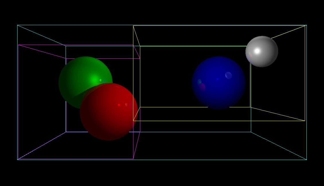
Next we figure out how to map pixels on the canvas to a viewport points, and then the magic starts. In real life the light is first emmitted from the light source and then it travels into our eyes, while reflecting from the objects. However when tracing rays, this process is reversed - we emit rays of light from the camera, going through a viewport until they hit the objects.

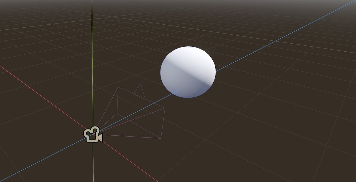basic scene with camera, viewport and an object

Project Setup

I’ve decided to go with C++ while following the book examples and extending it with my own implementation. To match the simplicity of the examples in the book, I’m also avoiding any external libraries. When it came to showing the results, I thought why bother drawing them on the screen - maybe a BMP image would be quite straightforward to implement instead, and it actually is :)

Whole Raytracer implementation can be found on my Github split into separate chapters to follow the progress.

Tracing Rays

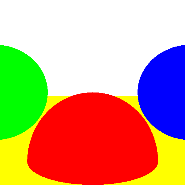
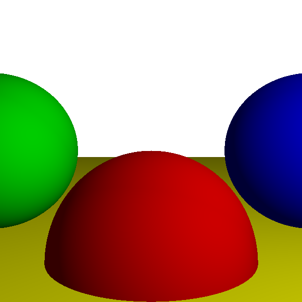
Now after we setup the project and our scene is ready, we’ll drop a few objects in it, and you guessed it, it’s gonna be spheres! Once we emit a ray, the tracing algorithm goes through each object in the scene and calculates the intersection between the ray and the object. We emit a ray for every pixel on the canvas starting from the camera position since we’re not interested in the objects behind the camera. The first result just shows the colors of the objects (green, red, blue and yellow spheres), so they look pretty flat.

basic raytracing

Lights and Shadows

We improve it by first introducing a concept of light and defining three sources:

• Point light has a position in 3D space, emits light equally in every direction.
• Directional light has no position, emits light in a single direction.
• Ambient light contributes some light to every point in the scene.

These sources of light are designed to resemble a very simplified version of how light works in the real world, however it is good enough to create an illusion which can be computed with nowadays hardware.

Next we need to specify how these lights interact with the objects in our scene. For simplicity, we classify objects into matte and shiny ones, which sets the way they reflect the lights.

• Diffuse Reflection - a process of scattering of light from a matte surface in many directions.
• Specular Reflection - mirror-like reflection of light from a shiny surface, where light rays reflect at the same angle they hit the surface.

We apply both diffuse and specular reflection to the objects by specifying their specular exponent.

Now that we have lights, we should have shadows to make scene look more realistic. Shadow basically means a spot where a light couldn’t reach because of another object in the way. Since we’ve agreed to have ambient light everywhere in the scene, shadows will be affecting directional and point lights. The algorithm is pretty simple - before calculating the lighting of the object we check if there’s any obstructing object in front of it following a direction of light. And if there’s one, then we don’t proceed with lighting calculations.

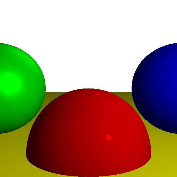
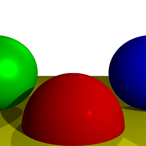
This is the first time we’ve made objects interact with each other and result looks quite impressive, given that we’re mostly relying on a few vector operations!

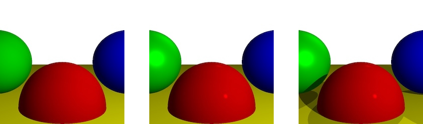diffuse reflection > specular reflection > shadows

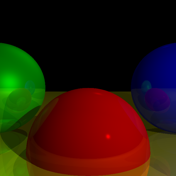
Reflections

Now that we have shiny objects and objects interacting with each other, we can implement a proper reflection. For that we’ll need to add a new property to specify how much reflective objects are, in a range 0…1. And in order to implement the way we trace a ray when it hits a reflective surface, we need to calculate the mirrored vector and trace the ray recursively. However recursion should stop at some point, and we need a way to exit it in case our ray is stuck between reflective surfaces. So we introduce a number of recursive raytracing operations we can do before we stop. Finally, a reflective surface can have its own color, so we blend these colors by computing weighted average of the surface color and reflected color.

Now that’s where I started experiencing differences from the original implementation. First is appearance of a shadow acne artefact after adding a reflections implementation. And you can see it’s mostly happening on the big yellow sphere because it looks almost flat, and the rays could be bouncing off the surface and recursively hitting it again caused by a floating point error. You see, since JS is used for the books examples, it has double-precision numbers, while I’m using a single-precision float in my C++ implementation, which can be more sensitive to small floating point errors. To fix it, I introduced a small epsilon padding every time we recursively trace a ray to calculate reflections, so that the ray would originate slightly above the surface.

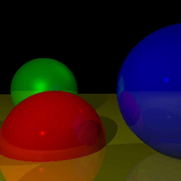
Another thing I’ve noticed was light reflections on the green and red spheres were slightly different in my implementation. The reason for that was that I was using uint8_t to represent the color values with 0…255 range which seemed quite logical to me in the beginning. However it didn’t produce the same smooth gradients sometimes, so I switched to float with 0…1 range and the issue was fixed, because the colors wouldn’t get clamped during computations until we need to render the final result.

And honestly I’m impressed - the whole implementation so far takes less than 300 loc, and runs in 50 ms on my machine.

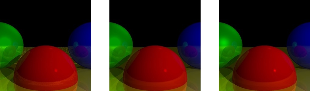shadow acne > clamped colors > final reflections

Extending the Raytracer

Here starts the fun part where we’re on our own. There’re few ideas/exercises in the book for us to implement, so we can extend our Raytracer with more features and think of a few optimization techniques. However my goal is not to squeeze the performance out of it, but rather to learn, observe and play around. So far it’s all running on a CPU in a single thread :)

Subsampling

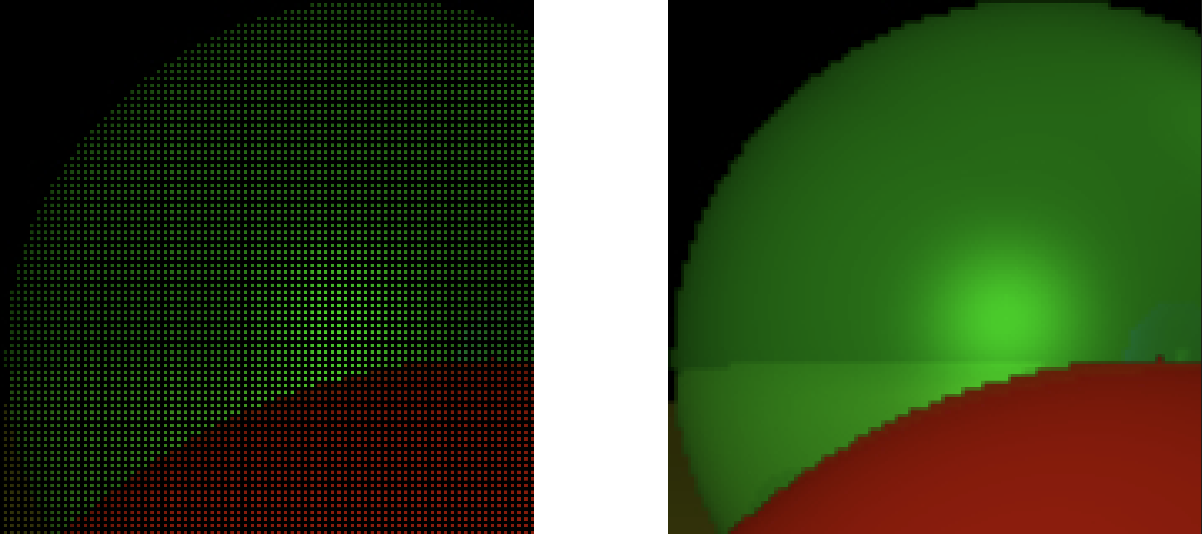
One way to optimize performance is by using a subsampling the scene. It’s a tradeoff - we can trace less rays to save computation costs but in return we’ll need to interpolate the missing colors based on the neighbors which might not end up in a crispy result. I decided to skip every other row and column when tracing rays and then simply come up with an average color between the known neighbors.

During interpolation I will start with an offset and also skip every other row and column so I can visit missing colors. You can image being in the center X surrounded by known colors in the corners and having top, bottom, right, left and center colors empty for now. In our algorithm we’re moving from the bottom left corner to the top right corner when iterating through the image. So in order to not calculate same colors twice, we only need to interpolate left, bottom and center colors on every interation and only when we hit the borders of the image we’ll do the top and right ones. Left color is based on its top and bottom neighbors, bottom color is based on its left and right neighbors, and center color is based on its four corner neighbors. Colors are mixed by simply getting an average color.

┌─────┐   ┌─────┐     ┌─────┐   ┌─────┐
│■ □ ■│   │■ □ ■│     │■ □ ■│   │■ □ ■│
│□ X □│ > │■ ■ □│ ==> │□ X □│ > │■ ■ □│ ==> ...
│■ □ ■│   │■ ■ ■│     │■ □ ■│   │■ ■ ■│
└─────┘   └─────┘     └─────┘   └─────┘

So the results on my machine are following - before subsamplingit it took ~52ms and after subsampling it takes ~22ms, which is not 4x but still quite a speed-up!

sampling + interpolation

Bounding Volume Hierarchy

Right now, in order to check if a ray intersects with an object, we need to go through all the objects in the scene for each ray and calculate whether they intersect while figuring out the closest of them to the camera. It sounds like a lot of work especially when there’re hundreds or thousands of objects in the scene.

Imagine if we could divide our scene into zones which would group the objects that spatially belong there, and instead of traversing every single object, we would travers zones first. If a ray hits one of the zones, then we can only check the objects inside of it. It sounds like a drastic improvement if for 1000 of objects we have i.e. 10 zones, where each has ~100 objects. Of course we can go deeper and divide those zones further and further. And it looks like a tree data structure would fit well here, which is in fact called a bounding volume hierarchy tree (BVH Tree).

In order to build such a tree, we first need to feed it the objects from the scene. It will create a box which perfectly fits those objects so that it becomes easier to compute whether the ray even hits the area with objects. Then it starts splitting the box into smaller boxes by the longest axis (x, y or z). The box is called an axis-aligned bounding box (AABB). The objects get sorted by their centroids on the splitting axis, then divided in half and are moved to the left and right sub-boxes (BVH tree nodes). The process repeats until we either hit the limit of splitting levels or the minimum amount of objects per AABB.

Figuring out the ray intersection is relatively simple. We first check if the ray hits a root AABB of the tree, then we go deeper into nodes of the tree by checking their AABBs intersections until we actually hit leaf nodes. Inside the leaf node we check for an intersection with its AABB and its objects by figuring out the closest one. Since we were always halving the nodes, there’s always left and right child node, so if both of them have been intersected by a ray, then we compare which of their hit objects is closer to the camera and return it as a result. You can imagine there might be as well only one leaf’s object hit or even none at all.

bounding volume hierarchy tree

Implementing it in C++ was more or less straightforward. This whole time we were working with spheres only, however next exercise encourages us to implement another shape. Which is why I’ve introduced an Object abstraction and a HitInfo structure which contains necessary info to render the object hit by ray. As per ownership, scene is the owner of both - the BVH tree via a unique_ptr and the objects as a vector<unique_ptr<Object>>, while the tree references objects through const Object*.

Triangles

Supporting an additional shape wasn’t a difficult task. Since BVH already works with Object abstraction, we only need to conform Triangle to it and implement bounds and intersection methods. When implementing bounds it’s good to take a small epsilon padding into account to avoid floating point errors. And as for the intersection computation I went with Möller-Trumbore algorithm and have learnt about barycentric coordinates and the fun things you can do using simple weights.

supporting triangles

Constructive Solid Geometry

Sounds fancy, right? Really you can think of it as applying set operations to the objects.

In this case we’re implementing three operations - union, intersection and difference:

• Union would be the most intuitive - you end up with a combination of two objects.
• Intersection you can imagine resulting in a lense when you intersect two spheres.
• Difference could be thought of a bite from an apple (or a young moon) - you remove a part from the original object by diffing with a second object.

Implementing it was a lot of fun, because it looks like a quite difficult task to do with geometric shapes, however there’s a trick which allows to achieve it by a few simple operations.

Previously in order to trace a ray to an object, we’d only need its closest hit point with the object in order to get its color. This time we’ll collect both - a point where the ray enters the object and a point where it exits the object (t-min and t-max).

Imagine we have two overlapping objects A and B with their following t-min and t-max values:

                             A
A object:             ┌─────────────┐
  * t-min: t0         │       ┌─────┼───────┐
  * t-max: t2         │       │     │       │
                     t0      t1    t2      t3
                 ─────╬───────╬─────╬───────╬────▶
B object:             │       │     │       │
  * t-min: t1         └───────┼─────┘       │
  * t-max: t3                 └─────────────┘
                                     B

Next, we can represent set operation between the objects as set operations between their t-min and t-max ranges, as shown below. The resulting t-min and t-max range will be the one to define the resulting object.

        t0          t1   t2          t3
    A ───┼████████████████┼───────────┼───

    B ───┼───────────┼████████████████┼───

A ∪ B ───┼████████████████████████████┼───

A ∩ B ───┼───────────┼████┼───────────┼───

A - B ───┼███████████┼────┼───────────┼───

CSG Refactoring

Implementing a Constructive Solid Geometry (CSG) required another refactoring of the existing code due to the following requirements:

1. A resulting CSG object should included into BVH Tree as a single object.
2. A resulting CSG object should participate in another CSG operations.
3. A resulting CSG object preserves material properies from only one of the two objects participating in the CSG operation.
4. Not all objects can participate in CSG - i.e. spheres can as they’re solid objects, but triangles can’t since they only belong to a plane.

Initially we had an Object to abstract Sphere and Triangle, and a HitInfo to keep the information when a ray hits an object. Meanwhile Object is a mix of geometry (centroid, bounds, intersection) and appearance (color, specular exponent, reflective value).

struct HitInfo {
    Vec3 point, normal;
    float t;
    const Object* object;
};

struct Object {
    float specular, reflective;
    Color color;

    virtual AABB bounds() const = 0;
    virtual Vec3 centroid() const = 0;
    virtual optional<HitInfo> intersect(const Ray& ray, float t_min, float t_max) const = 0;
}

struct Sphere : Object { ... }
struct Triangle : Object { ... }

As we’re introducing CSG - it’s mostly about geometry, and having objects with appearance is redundant, as appearance can be figured out on a later stage. One way to address this is to split Object into Shape and Material. Now we can have entirely geometrical operations, and we can connect material to a shape later on. HitInfo can be renamed into ShapeHit and contain only geomertical info of a ray hitting a shape. However there’s still one issue here - we need to allow only certain shapes to participate in the CSG, and since I like relying on the type system more than runtime logic when possible, I decided to introduce a SolidShape descendant of the Shape to be handled by the CSG. We keep a shared_ptr reference to the left and right shapes inside a CSGShape in case same shape wants to participate in multiple CSG shapes.

struct ShapeHit {
    Vec3 point, normal;
    float t;
};

struct Shape {
    virtual AABB bounds() const = 0;
    virtual Vec3 centroid() const = 0;
    virtual optional<ShapeHit> intersect(const Ray& ray, float t_min, float t_max) const = 0;
};

struct SolidShape : Shape {}

struct Sphere : SolidShape { ... }
struct Triangle : Shape { ... }

struct CSGShape : SolidShape {
    shared_ptr<SolidShape> left, right;
    CSGOperation operation;
    ...
}

Next phase is to combine geometry and appearance into an abstraction which BVH tree and our existing raytracing logic can work with. On the first sight it might look like BVH tree is purely geomertic - built purely based on geometry, and computing intersection purely based on geometry. However in practice it’s more convenient when we get appearance along with a ray hit info so we don’t need to do any additional deductions later on how to get material properties out of the purely geometric hit info. Hence we want to keep BVH tree working with an abstraction which combines geometry and appearance together.

We can introduce a Primitive to combine Material and Shape, and a PrimitiveHit to combine ShapeHit and Material for the rendering part. A primitive hit inherits the shape hit and adds a non-owning reference to a material on top of it. We can also make a material selection a bit more dynamic when we compute intersection here, i.e. a CSG might want to decide which material to pick based on the hit details, while simpler shapes can just resolve to a single material. So our Primitive abstraction can be initialized with a selector to resolve a Material.

struct Material {
    float specular;
    float reflective;
    Color color;
};

struct PrimitiveHit : ShapeHit {
    const Material* material  = nullptr;
};

struct Primitive {
    shared_ptr<Shape> shape;
    function<const Material&(const ShapeHit&)> material;
    ...
    optional<PrimitiveHit> intersect(const Ray& ray, float t_min, float t_max) const {
        if (auto s_hit = shape->intersect(ray, t_min, t_max)) {
            return PrimitiveHit(*s_hit, &material(*s_hit));
        }
        return nullopt;
    }
}

CSG Algorithm

Second part of CSG implementation is the actual intersection algorithm. We can informally call it event-walking since we’re walking along the ray through a list of intersection events (enter/exit).

At each step of the iteration, we first pick the nearest intersection (event) by comparing the hits from the left and right child shapes. Next we the figure out whether the ray is entering or exiting those shapes. And based on that we apply the set operation (union, intersection or difference) to figure out if we’re inside or outside of the combined CSG shape. We advance to whichever intersection (left or right) is closer along the ray. This ensures we walk through the events in the increasing t order. And if the state of the combined CSG shape is switching from outside -> inside, it means that we’ve found the hit of the visible boundary of the resulting surface.

When advancing through the loop iterations, we add a small epsilon padding to the next_t_min to avoid floating point error overlaps.

And in case of a difference operation, we should flip the hit’s normal in case we’re showing the cavity side. Originally that shape’s (right child’s) normal is facing outward, however after it was used to cut out a part of another object (left child), we’re showing its “inside wall” now, hence the normal direction should be the opposite.

constructive solid geometry

Transparency

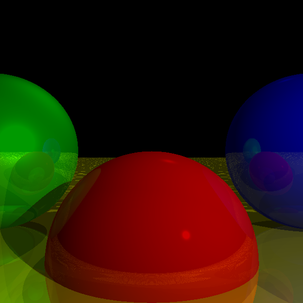
And now we’re coming to the final Raytracer extension here - adding transparency and refraction. Implementing it didn’t seem like a lot of work - it’s quite similar to reflection just a different formula. However it took me some time to figure it out to a satisfying result.

• In order to implement refraction we go with Snell’s law, however it seems more geometric while we’re working with direction vectors, not explicit angles, so it had to be adjusted a bit (vector operations use cos instead of sin).
• Next, we are mixing reflection with transparency (also semi-transparent materials with their own colors) and refraction - which made it difficult to debug at first.
• And finally we’re met with reflecting transparent primitives from other primititves, and seeing transparent primitives through other transparent primitives.

So to simplify things, I removed reflection and focused only on pure transparency once the refraction formula was done. Then I started adding material’s own color to the transparency and checking if semi-transparency works fine. And in order to blend colors, we first need to normalize them to avoid oversaturation, and then blend together reflection color + refraction color + local object’s color as a good old weighted average of those colors.

Now when I thougt everything was working properly I’ve noticed that some objects in reflections lack details which took me some time to debug the code only to figure out the recursion_depth argument which I’ve completely forgotten of :D It basically controls how many times we can recursively trace a ray when it reflects off of an object or refracts through it. However increasing recursion_depth level leads to more computations needed to render a picture, hence it’s a tradeoff between speed and a satisfacting amount of details.

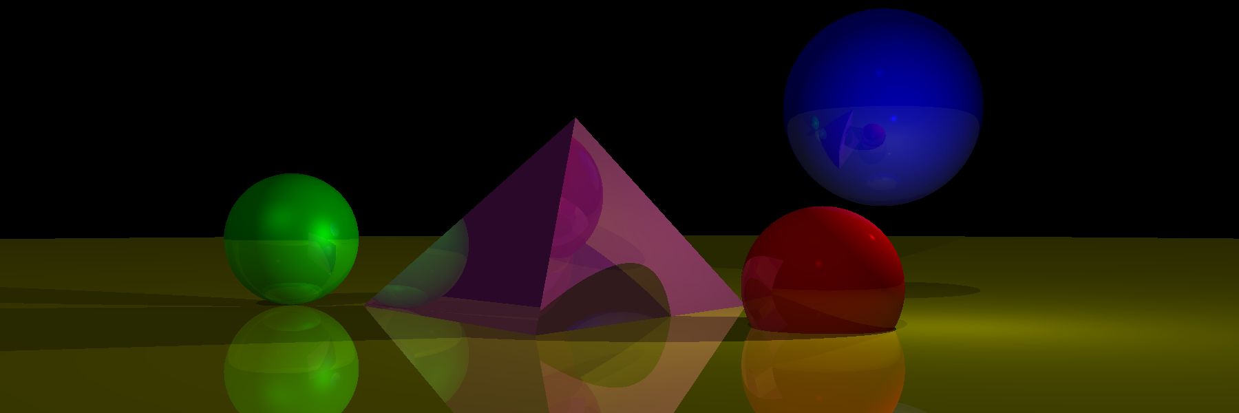
To demosntrate how transparency works I’ve created two objeects:

• Magnifying lens (on top of triangles) built using CSG by itersecting two spheres, it is a completely transparent material with a refraction value of 1.5.
• Fishbowl sphere with refraction of 1.1 and transparcy of 0.8, and a cyan color.

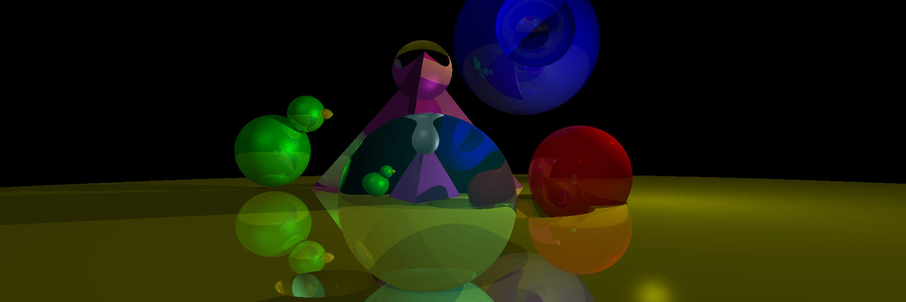With a recursion depth of 2 you can see some details in reflections, but already flat objects in refraction.

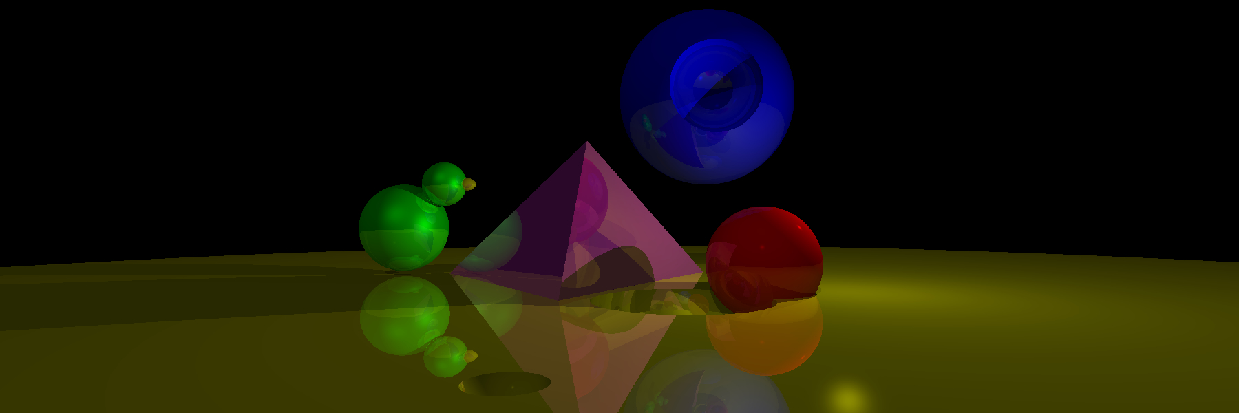
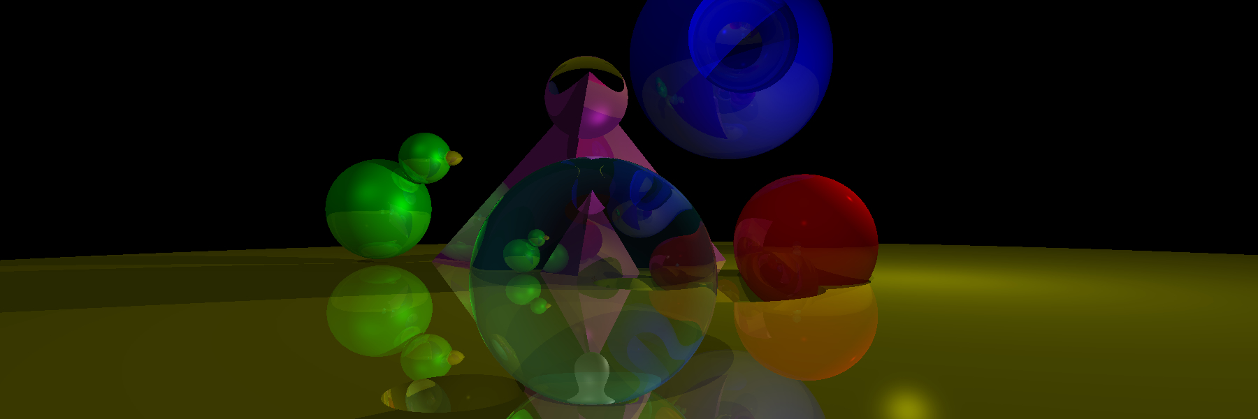By increasing recursion depth to 3 it already looks good but we loose lense details in its reflection from a yellow ball which we observe through a fishbowl refraction.

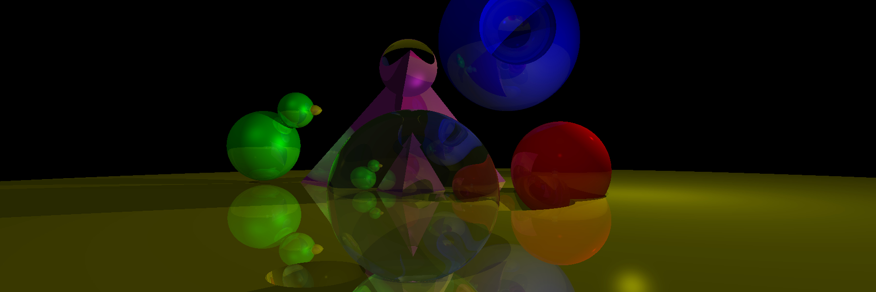And with a recursion depth of 4 we can see a decent amount of details.

Conclusion

In conclusion I had a lot of fun learning and building a Raytracer. It helped me to practice with vector operations, feel a bit more confident in 3D space, and look behind the curtains of the computer graphics magic ✨

Links

• Computer Graphics from Scratch
• My Implementation on Github